
Companion to: Guajardo-Leiva et al., Seasonal structuring of microbial communities and functional potential in a Patagonian fjord
This walkthrough explains the logic behind each analysis in the paper — not just how the code works, but why we made each analytical choice and what the results mean biologically. It is written for anyone familiar with R and community ecology who wants to understand or reproduce the work, or adapt it to their own system. All scripts and data files are available in this repository.
Data and scripts: All files needed to reproduce the analyses are available at github.com/ecastron/comau-reproducibility. Download the repo as a ZIP (green Code button) or clone it:
git clone https://github.com/ecastron/comau-reproducibility.gitThen run any figure script from that directory:
setwd("path/to/comau-reproducibility")
source("utils.R")          # always load this first
source("Figure1_final.R")  # or Figure2_final.R, etc.
The code chunks below are drawn directly from those scripts and are complete enough to reproduce each analysis step-by-step.
The story in one paragraph
Comau Fjord (42°S, Chilean Patagonia) is a deep, stratified fjord with a sharp two-layer water column: a shallow, freshwater-influenced surface layer (5 m) that swings wildly with season, and a deeper, saline layer (20 m) that barely changes. We sequenced the microbial community across both depths during three Southern Hemisphere seasons — Summer, Fall, Winter — and reconstructed 513 metagenome-assembled genomes (MAGs). The central question was whether depth and season structure communities in the same way or through different mechanisms. The answer is that they do not: surface communities are shaped by competition and niche partitioning (functionally diverse, phylogenetically overdispersed), while deep communities are shaped by environmental filtering (functionally convergent, phylogenetically clustered). pH emerges as the single strongest continuous driver, and seasonal timing — not geographic distance — best predicts how similar any two samples are.
Study system and prior work
Comau Fjord stretches ~45 km through northern Chilean Patagonia, reaching nearly 490 m depth. High rainfall and snowmelt create a shallow brackish surface layer over a cold, saline body of modified Subantarctic water. This stratification creates steep vertical gradients in temperature, salinity, nutrients, and pH. Salinity-driven stratification has been shown to shape macrobenthic biodiversity patterns along both the horizontal and vertical axes of the fjord Villalobos et al. 2021, and the same two-layer structure likely sets the template for the microbial niche partitioning we document here.
The metagenomes and MAGs used in this study were first described in Castro-Nallar et al. 2023, presenting the spatially and temporally resolved dataset as a resource. An earlier metagenomics survey by Guajardo-Leiva et al. 2023 established that surface communities are taxonomically distinct from global ocean surveys (Tara Oceans), yet converge on cosmopolitan marine lineages (Proteobacteria, Bacteroidota, Actinobacteria). The first metagenomic description of the fjord dates to a microbial mat study by Ugalde et al. 2013, which identified sulfate and nitrate reduction genes in Gammaproteobacteria-dominated communities — foreshadowing the sulfur-cycle signal we detect in the water column.
Salmon aquaculture: an elephant in the fjord
The northern Chilean Patagonian fjords, including Comau, host one of the world’s most intensive salmon aquaculture industries. Microcosm experiments conducted directly in Comau Fjord showed that nutrient loading from fish farms significantly restructures bacterial communities — dissimilarity between low- and high-nutrient treatments reaching 78% — while diversity itself remained resilient Olsen et al. 2017. Dissolved organic matter from salmon feed (SF-DOM) is highly reactive, boosting bacterial production 2-fold while reducing species richness Montero et al. 2022. Communities carry elevated antibiotic resistance genes (ARGs) — dominated by beta-lactams, tetracyclines, and MLS resistance Guajardo-Leiva et al. 2023. In March 2021, the same seasonal forcing that drives natural community dynamics triggered a catastrophic Heterosigma akashiwo bloom that killed ~6,000 tonnes of farmed salmon within 15 days Díaz et al. 2022.
Seasonal forcing in Patagonian fjords
Primary production in Chilean fjords swings by two orders of magnitude between winter and spring, with bacterioplankton tightly coupled to phytoplankton throughout Montero et al. 2011. In Puyuhuapi Fjord, Flavobacteriaceae, Rhodobacteraceae, and Cryomorphaceae dominate surface communities and their diversity declines with rising winter temperatures — a warning for climate change impacts Gutiérrez et al. 2018. Across a wider spatial scale, Tamayo-Leiva et al. 2021 showed that estuarine water influence structures bacterioplankton over hundreds of kilometres, with dissolved oxygen and salinity as first-order drivers.
Data objects and shared utilities
All analyses start from two core files and a shared utility script:
| File | Contents |
|---|---|
Comau_ps90.RDS | A phyloseq object: count table (MAGs × samples), taxonomy, sample metadata, and a rooted ML phylogeny built from 81 universal marker genes (IQ-TREE) |
gene_bin_mat.collapsed.v6.csv | Binary matrix of functional gene hits (rows = genes/KOs, columns = 677 MAGs before dereplication) |
utils.R | Shared palettes, season classifier, load_ps(), VIF filter, MRM wrappers |
Every script begins with source("utils.R"), which sets the working directory, defines palettes and helpers, and exposes load_ps(). Key definitions from utils.R:
# Season assignment — Southern Hemisphere calendar
get_season_sh <- function(d) {
  m <- as.integer(format(as.Date(d), "%m"))
  ifelse(m %in% c(12, 1, 2), "Summer",
         ifelse(m %in% c(3, 4, 5), "Fall",
                ifelse(m %in% c(6, 7, 8), "Winter", NA_character_)))
}

# Canonical palettes (Wong 2011 — colour-blind safe)
pal_season  <- c("Summer" = "#E69F00", "Fall" = "#D55E00", "Winter" = "#56B4E9")
shape_depth <- c("5" = 16, "20" = 17)

# Load and annotate phyloseq object
load_ps <- function(path = "Comau_ps90.RDS") {
  ps <- readRDS(path)
  sd <- as.data.frame(phyloseq::sample_data(ps))
  sd$Collection_Date <- as.Date(sd$Collection_Date)
  sd$season  <- factor(get_season_sh(sd$Collection_Date), levels = c("Summer", "Fall", "Winter"))
  sd$depth_m <- factor(as.character(sd$depth_m), levels = c("5", "20"))
  phyloseq::sample_data(ps) <- phyloseq::sample_data(sd)
  ps
}

# Iterative VIF filter (drops highest-VIF predictor until all VIF ≤ thr)
drop_high_vif_vegan <- function(Xdf, Y, thr = 10) {
  keep <- colnames(Xdf)
  repeat {
    mod <- vegan::rda(as.matrix(Y) ~ ., data = as.data.frame(Xdf[, keep, drop = FALSE]))
    v   <- vegan::vif.cca(mod)
    if (max(v, na.rm = TRUE) > thr && length(keep) > 1)
      keep <- setdiff(keep, names(which.max(v)))
    else break
  }
  Xdf[, keep, drop = FALSE]
}
Figure 1 — Who is there, and does it change with season?
Script: Figure1_final.R
This figure establishes the basic pattern: season structures the community (PCoA + PERMANOVA), the phylum composition is depth-stratified and seasonally dynamic, and phylogenetic relatedness (aMPD) varies across season × depth combinations.
Panel A — Map
The 12 sampling sites span the length of Comau Fjord, with Huinay Research Station as the base. The map uses GADM Chile administrative shapefiles and rnaturalearth for the locator inset.
source("utils.R")
library(sf); library(rnaturalearth); library(ggrepel); library(ggspatial)
library(shadowtext); library(readr); library(ggplot2)

# Helper: 5-pointed star polygon at lon/lat
make_star_lonlat <- function(lon, lat, r_deg = 0.010, inner_ratio = 0.5, n = 5) {
  lat_rad <- lat * pi/180
  ang <- seq(0, 2*pi, length.out = 2*n + 1)[-(2*n + 1)]
  rad <- rep(c(r_deg, r_deg*inner_ratio), n)
  dx  <- (rad * cos(ang)) / max(0.1, cos(lat_rad))
  dy  <-  rad * sin(ang)
  data.frame(long = lon + dx, lat = lat + dy, group = "huinay_star")
}

meta  <- readr::read_tsv("metadata.tsv", show_col_types = FALSE)
pts12 <- meta |>
  transmute(line_chr = gsub("^L", "", as.character(line)),
            site_chr = gsub("^S", "", as.character(site)),
            longitude = as.numeric(longitude),
            latitude  = as.numeric(latitude)) |>
  filter(is.finite(longitude), is.finite(latitude)) |>
  group_by(line_chr, site_chr) |>
  summarise(longitude = median(longitude), latitude = median(latitude), .groups = "drop") |>
  mutate(label = paste0("L", line_chr, "S", site_chr))

adm2        <- sf::st_read("CHL_adm_shp/CHL_adm2.shp", quiet = TRUE) |> sf::st_transform(4326)
palena_wgs  <- dplyr::filter(adm2, NAME_2 == "Palena")
huinay      <- data.frame(longitude = -72.415246, latitude = -42.379839)
huinay_star <- make_star_lonlat(huinay$longitude, huinay$latitude, r_deg = 0.008)
chl         <- rnaturalearth::ne_countries(country = "Chile", returnclass = "sf") |>
                 sf::st_transform(4326)

# Bounding box for main map
pad_x <- 0.05; pad_y <- 0.03
xlim  <- c(min(pts12$longitude) - pad_x, max(pts12$longitude) + pad_x)
ylim  <- c(min(pts12$latitude)  - pad_y, max(pts12$latitude)  + pad_y)

main_map <- ggplot() +
  geom_polygon(data = ..., aes(x = long, y = lat, group = group),   # palena_df
               color = "grey35", fill = "grey95", linewidth = 0.6) +
  geom_polygon(data = huinay_star, aes(x = long, y = lat, group = group),
               fill = "black", color = "black") +
  geom_point(data = pts12, aes(x = longitude, y = latitude),
             shape = 21, fill = "red", color = "black", size = 3.4) +
  ggrepel::geom_label_repel(data = pts12, aes(x = longitude, y = latitude, label = label),
                            size = 3.2, fill = "white", label.size = 0, seed = 42) +
  coord_sf(xlim = xlim, ylim = ylim, expand = FALSE) +
  annotation_north_arrow(location = "tl", style = north_arrow_minimal()) +
  annotation_scale(location = "bl") +
  theme_minimal()

locator <- ggplot() +
  geom_sf(data = chl, fill = "grey95", color = "grey35", linewidth = 0.3) +
  geom_sf(data = palena_box, fill = NA, color = "red", linewidth = 0.6) +
  coord_sf(expand = FALSE) + theme_void()

p_A <- main_map +
  patchwork::inset_element(locator, left = 0.04, bottom = 0.06, right = 0.42, top = 0.46)
Panel B — Beta-diversity (PCoA + PERMANOVA)
We compute Bray–Curtis dissimilarity on relative abundances. Bray–Curtis is bounded [0,1], insensitive to joint absences, and the standard choice for compositional community data. The PERMANOVA is stratified by depth so that samples are only shuffled within depth groups — this holds depth constant and isolates the seasonal signal.
ps     <- load_ps()
ps_rel <- transform_sample_counts(ps, function(x) if (sum(x) > 0) x/sum(x) else x)
dist_mat <- phyloseq::distance(ps_rel, method = "bray")
set.seed(1)
ord  <- ordinate(ps_rel, method = "PCoA", distance = dist_mat)
pdat <- plot_ordination(ps_rel, ord, justDF = TRUE)

p_B <- ggplot(pdat, aes(x = Axis.1, y = Axis.2)) +
  geom_point(aes(color = season, shape = depth_m), size = 2.2, alpha = 0.9) +
  stat_ellipse(aes(color = season, group = season), type = "t", level = 0.95) +
  scale_color_manual(values = pal_season) +
  scale_shape_manual(values = shape_depth) +
  theme_bw(base_size = 11)

# Stratified PERMANOVA (strata = depth holds depth constant)
meta    <- as(sample_data(ps_rel), "data.frame")
meta    <- meta[attr(dist_mat, "Labels"), , drop = FALSE]
keep    <- !is.na(meta$season) & !is.na(meta$depth_m)
meta    <- meta[keep, ]; dmat <- as.matrix(dist_mat)[keep, keep]
adon    <- vegan::adonis2(dmat ~ season, data = meta, permutations = 999, strata = meta$depth_m)
# Result: R² = 0.273, P = 0.001

# Pairwise contrasts (BH-corrected)
pairwise_permanova_strat <- function(dmat, meta, group_col = "season",
                                     strata_col = "depth_m", permutations = 999) {
  g  <- droplevels(meta[[group_col]]); lv <- levels(g)
  out <- list(); k <- 1
  for (i in seq_len(length(lv)-1)) for (j in (i+1):length(lv)) {
    pair <- c(lv[i], lv[j]); idx <- g %in% pair
    fit  <- vegan::adonis2(dmat[idx,idx] ~ meta[[group_col]][idx],
                           permutations = permutations, strata = meta[[strata_col]][idx])
    tab  <- as.data.frame(fit)
    out[[k]] <- data.frame(Comparison = paste(pair, collapse=" vs "),
                           R2 = tab$R2[1], p = tab$`Pr(>F)`[1])
    k <- k+1
  }
  df <- do.call(rbind, out)
  df$`p (BH)` <- p.adjust(df$p, method = "BH")
  df
}
pw_df <- pairwise_permanova_strat(dmat, meta)
Season explains 27% of community variation. All pairwise seasonal contrasts are significant after BH correction, with Summer–Fall showing the largest divergence (R² = 0.316).
Panel C — Phylum-level seasonality
Raw counts are aggregated to phylum, then plotted as stacked area charts across calendar month-day (so all years overlay on the same axis). Only phyla contributing ≥ 1% of total counts are shown individually.
mat_counts <- as(otu_table(ps), "matrix")
if (!taxa_are_rows(ps)) mat_counts <- t(mat_counts)

phy_vec    <- as.vector(tax_table(ps)[, "Phylum"])
phy_vec[is.na(phy_vec) | phy_vec == ""] <- "Unclassified"
names(phy_vec) <- rownames(tax_table(ps))
mat_phylum <- rowsum(mat_counts, group = phy_vec, reorder = TRUE)

smeta <- as(sample_data(ps), "data.frame") %>%
  tibble::rownames_to_column("Sample") %>%
  mutate(Collection_Date = as.Date(Collection_Date),
         cal_date = as.Date(paste0("2000-", format(Collection_Date, "%m-%d"))),
         depth_m  = factor(as.character(depth_m), levels = c("5","20")))

dfC <- as.data.frame(t(mat_phylum)) %>%
  tibble::rownames_to_column("Sample") %>%
  pivot_longer(-Sample, names_to = "Phylum", values_to = "Count") %>%
  left_join(smeta, by = "Sample") %>%
  filter(!is.na(cal_date), !is.na(depth_m))

# Keep phyla ≥ 1% globally
dom_phyla <- dfC %>%
  group_by(Phylum) %>% summarise(Total = sum(Count), .groups = "drop") %>%
  mutate(Prop = Total / sum(Total)) %>%
  filter(Prop >= 0.01) %>% pull(Phylum)

dfC <- dfC %>%
  mutate(PhylumCollapsed = if_else(Phylum %in% dom_phyla, Phylum, "Other"),
         PhylumCollapsed = factor(PhylumCollapsed, levels = names(pal_phylum)))

df_day <- dfC %>%
  group_by(cal_date, depth_m, PhylumCollapsed) %>%
  summarise(Count = sum(Count, na.rm = TRUE), .groups = "drop")

p_C <- ggplot(df_day, aes(x = cal_date, y = Count, fill = PhylumCollapsed)) +
  geom_area(position = "fill", linewidth = 0.1) +
  facet_wrap(~ depth_m, ncol = 1,
             labeller = labeller(depth_m = c(`5` = "5 m", `20` = "20 m"))) +
  scale_y_continuous(labels = scales::percent_format(accuracy = 1)) +
  scale_x_date(date_labels = "%b", date_breaks = "1 month") +
  scale_fill_manual(values = pal_phylum, drop = TRUE) +
  labs(x = "Calendar date", y = "Relative abundance", fill = "Phylum") +
  theme_bw(base_size = 11)
A notable finding: the Cyanobacteria bloom from April to August at 5 m — Southern Hemisphere mid-year, when the mixed layer deepens and nutrients surge. This mirrors bacterioplankton–phytoplankton coupling patterns documented in Reloncaví Fjord Montero et al. 2011.
Panel D — Abundance-weighted MPD
To measure not just who is there but how related they are, we compute abundance-weighted mean pairwise distance (aMPD). Statistical testing uses aligned-rank transform ANOVA (ARTool) — appropriate for non-normal data in a two-way factorial design (season × depth). Post-hoc Dunn tests are run separately within each depth to avoid confounding depth differences with seasonal contrasts.
library(picante); library(ARTool); library(rstatix); library(multcompView)

comm <- as(otu_table(ps), "matrix")
if (taxa_are_rows(ps)) comm <- t(comm)
comm <- comm[rowSums(comm) > 0, , drop = FALSE]

tree       <- phy_tree(ps)
tax_in_both <- intersect(colnames(comm), tree$tip.label)
comm       <- comm[, tax_in_both, drop = FALSE]
tree       <- ape::keep.tip(tree, tax_in_both)
comm_rel   <- sweep(comm, 1, rowSums(comm), "/")

D    <- cophenetic(tree); D <- D[colnames(comm_rel), colnames(comm_rel)]
aMPD <- picante::mpd(samp = comm_rel, dis = D, abundance.weighted = TRUE)

sd2 <- as(sample_data(ps), "data.frame")
adiv_pd <- data.frame(Sample = rownames(comm_rel), aMPD = as.numeric(aMPD)) %>%
  left_join(tibble::rownames_to_column(sd2, "Sample")[, c("Sample","season","depth_m")],
            by = "Sample") %>%
  filter(!is.na(season), !is.na(depth_m))

# Two-way ART ANOVA
art_fit <- ARTool::art(aMPD ~ season * depth_m, data = adiv_pd)
anova(art_fit)

# Post-hoc: Dunn test within each depth
dunn_depth <- adiv_pd %>%
  group_by(depth_m) %>%
  rstatix::dunn_test(aMPD ~ season, p.adjust.method = "BH") %>%
  ungroup()

# Compact letter display per depth
letters_df <- dunn_depth %>%
  mutate(comp = paste(group1, group2, sep = "-")) %>%
  select(depth_m, comp, p.adj) %>%
  group_split(depth_m) %>%
  lapply(function(df) {
    vec <- setNames(df$p.adj, df$comp)
    L   <- multcompView::multcompLetters(vec, threshold = 0.05)$Letters
    tibble::tibble(season = names(L), .label = unname(L))
  }) %>%
  { bind_rows(mapply(function(df, d) mutate(df, depth_m = d),
                     ., unique(dunn_depth$depth_m), SIMPLIFY = FALSE)) }

p_D <- ggplot(adiv_pd, aes(season, aMPD, fill = season)) +
  geom_boxplot(width = 0.7, alpha = 0.85, outlier.shape = 21) +
  geom_jitter(width = 0.15, height = 0, size = 1.6, alpha = 0.6) +
  geom_text(data = letters_df,
            aes(x = season, y = max(adiv_pd$aMPD)*1.05, label = .label),
            inherit.aes = FALSE, vjust = 0, size = 3.4) +
  facet_grid(cols = vars(depth_m), drop = FALSE,
             labeller = labeller(depth_m = c(`5` = "5 m", `20` = "20 m"))) +
  scale_fill_manual(values = pal_season, drop = FALSE) +
  labs(x = NULL, y = "Abundance-weighted MPD") +
  theme_bw(base_size = 11) + theme(legend.position = "none")
Key finding: Fall communities at 5 m are phylogenetically more clustered than Summer or Winter — environmental filtering pulls the surface community toward closely related lineages during the productive autumn period.
Assembly and export
library(cowplot); library(ggplotify)

# Extract legends from B and C, remove from panels
leg_B <- cowplot::get_legend(p_B + theme(legend.position = "right"))
leg_C <- cowplot::get_legend(p_C + theme(legend.position = "right"))
p_B_clean <- p_B + theme(legend.position = "none")
p_C_clean <- p_C + theme(legend.position = "none")
p_D_clean <- p_D + theme(legend.position = "none")

# Render B (with PERMANOVA inset) to canvas for cowplot alignment
p_B_inset <- p_B_clean +
  patchwork::inset_element(tab_pw_plot, left=0.02, bottom=0.58, right=0.48, top=0.98)
p_B_canvas <- ggplotify::as.ggplot(function() print(p_B_inset))

# Align and assemble
bottom_right <- cowplot::plot_grid(p_C_clean, p_D_clean, ncol = 2,
                                   labels = c("C","D"), label_fontface = "bold")
right_col    <- cowplot::plot_grid(p_B_canvas, bottom_right, ncol = 1,
                                   labels = c("B", NULL), rel_heights = c(1.05, 1.00))
right_full   <- cowplot::plot_grid(right_col,
                                   cowplot::plot_grid(leg_B, leg_C, ncol = 1),
                                   ncol = 2, rel_widths = c(1, 0.20))
fig1 <- cowplot::plot_grid(p_A + labs(title = NULL), right_full,
                           ncol = 2, labels = c("A", NULL), rel_widths = c(1.15, 1.60))

ggsave("Figure1.pdf", fig1, width = 13, height = 9, units = "in", useDingbats = FALSE)
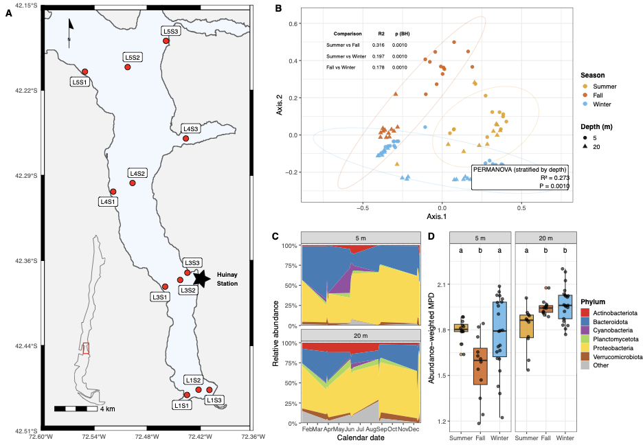
Figure 2 — Why do communities differ?
Script: Figure2_final.R
Figure 1 showed that communities differ by season; Figure 2 asks what environmental variables drive that variation, and whether the fjord is dispersal-limited or seasonally forced.
Collinearity filtering (VIF)
Environmental predictors in a fjord are highly collinear (temperature co-varies with salinity, nutrients co-vary with productivity). Before constrained ordination, we iteratively remove predictors with VIF > 10 using drop_high_vif_vegan() from utils.R. This leaves a set of largely independent variables whose individual contributions can be interpreted.
source("utils.R")
library(vegan); library(mgcv); library(ggtext)

ps   <- load_ps()
meta <- as(sample_data(ps), "data.frame") %>% tibble::rownames_to_column("SampleID")
meta$season  <- factor(meta$season, levels = c("Fall","Summer","Winter"))
meta$depth_m <- suppressWarnings(as.numeric(as.character(meta$depth_m)))

# Community (relative abundances, samples as rows)
Y_counts <- as(otu_table(ps), "matrix")
if (taxa_are_rows(ps)) Y_counts <- t(Y_counts)
rs    <- rowSums(Y_counts); rs[rs == 0] <- 1
Y_rel <- sweep(Y_counts, 1, rs, "/")

# Predictor groups
vars_nutrients    <- c("nitrate_uM","nitrite_uM","phosphate_uM","silicate_uM")
vars_physicals    <- c("salinity_PSU","temperature_C","pH")
vars_productivity <- c("chlorophyll_A_ugL","C_total_ug","N_total_ug","C_N_ratio")
vars_all <- unique(c(intersect(vars_nutrients, colnames(meta)),
                     intersect(vars_physicals, colnames(meta)),
                     intersect(vars_productivity, colnames(meta))))

X_num  <- as.data.frame(lapply(meta[, vars_all, drop=FALSE],
                               function(v) suppressWarnings(as.numeric(v))))
rownames(X_num) <- meta$SampleID
common <- intersect(rownames(Y_rel), rownames(X_num))
Y_rel  <- Y_rel[common,]; X_num <- X_num[common,]; meta <- meta[match(common, meta$SampleID),]
cc     <- complete.cases(X_num, meta$depth_m, meta$season)
Y_rel  <- Y_rel[cc,]; X_num <- X_num[cc,]; meta <- meta[cc,]
X      <- as.data.frame(scale(X_num))
X_vif  <- drop_high_vif_vegan(X, Y_rel, thr = 10)   # iterative VIF filter from utils.R
Panel A — Partial dbRDA
Distance-based redundancy analysis (capscale in vegan) is the constrained analogue of PCoA. Conditioning on depth and season partials them out so the plot shows only the residual environmental signal after removing those large effects.
env_partial  <- cbind(X_vif, depth_m = meta$depth_m, season = meta$season)
form_partial <- as.formula(
  paste("Y_rel ~", paste(colnames(X_vif), collapse = " + "),
        "+ Condition(depth_m) + Condition(season)")
)
mod_partial <- capscale(form_partial, data = env_partial, distance = "bray")

# Global test
anova(mod_partial, permutations = 999)
# adj. R² = 0.50, P = 0.001

# Term-by-term (marginal) significance
anova(mod_partial, permutations = 999, by = "term")

# Extract site and biplot scores for plotting
sc_sites <- scores(mod_partial, display = "sites", scaling = 2) %>% as.data.frame()
sc_bp    <- scores(mod_partial, display = "bp",    scaling = 2) %>% as.data.frame()
sc_sites$SampleID <- rownames(sc_sites)
plot_df  <- left_join(sc_sites, meta, by = "SampleID")

eig      <- mod_partial$CCA$eig
lab_x    <- sprintf("dbRDA1 (%.1f%%)", 100*eig[1]/sum(eig))
lab_y    <- sprintf("dbRDA2 (%.1f%%)", 100*eig[2]/sum(eig))
arrow_mul <- vegan:::ordiArrowMul(mod_partial, display = "bp")
sc_bp$arrow_x <- sc_bp$CAP1 * arrow_mul; sc_bp$arrow_y <- sc_bp$CAP2 * arrow_mul

p2A <- ggplot(plot_df, aes(x = CAP1, y = CAP2)) +
  geom_point(aes(color = season, shape = factor(ifelse(depth_m==5,"5 m","20 m"))),
             size = 2.5, alpha = 0.9) +
  scale_color_manual(values = pal_season) +
  scale_shape_manual(values = c("5 m" = 16, "20 m" = 17)) +
  geom_segment(data = sc_bp, aes(x=0, y=0, xend=arrow_x, yend=arrow_y),
               arrow = arrow(length = unit(0.25,"cm")), linewidth = 0.5) +
  ggrepel::geom_text_repel(data = sc_bp, aes(x=arrow_x, y=arrow_y, label=rownames(sc_bp)),
                           size = 3) +
  labs(x = lab_x, y = lab_y) + theme_bw(base_size = 11)
pH shows the strongest alignment in ordination space — ecologically meaningful because Comau’s deep waters are aragonite-undersaturated, and pH fluctuates seasonally as photosynthesis and respiration shift the carbonate equilibrium Garcia-Herrera et al. 2022.
Panel B — Unique variance fractions
Each predictor group’s unique contribution is estimated by conditioning on the other two groups plus depth and season. This partitions the explained variance into components attributable to nutrients, physical variables, and productivity.
fit_unique <- function(Y, X_main, X_condlist, extra_cond = NULL) {
  dat <- do.call(cbind, c(list(X_main), X_condlist,
                           if (!is.null(extra_cond)) list(extra_cond) else NULL))
  colnames(dat) <- make.unique(colnames(dat))
  k     <- ncol(X_main)
  form  <- paste("Y ~", paste(colnames(dat)[1:k], collapse=" + "),
                 "+ Condition(", paste(colnames(dat)[-(1:k)], collapse=" + "), ")")
  mod   <- capscale(as.formula(form), data = dat, distance = "bray")
  list(R2 = RsquareAdj(mod), anova = anova(mod, permutations = 999))
}

extra_cond <- data.frame(depth_m = meta$depth_m, season = meta$season)
X_N <- X_vif[, intersect(colnames(X_vif), vars_nutrients),    drop=FALSE]
X_P <- X_vif[, intersect(colnames(X_vif), vars_physicals),    drop=FALSE]
X_R <- X_vif[, intersect(colnames(X_vif), vars_productivity), drop=FALSE]

uN <- fit_unique(Y_rel, X_N, list(X_P, X_R), extra_cond)  # Physical adj.R² = 0.073
uP <- fit_unique(Y_rel, X_P, list(X_N, X_R), extra_cond)  # Nutrients adj.R² = 0.034
uR <- fit_unique(Y_rel, X_R, list(X_N, X_P), extra_cond)  # Productivity adj.R² = 0.017
Panel C — GAM responses to pH
The six MAGs most strongly aligned with the pH axis are identified from the dbRDA species scores (projection onto the pH biplot vector), then modelled with GAMs on CLR-transformed abundances. CLR transformation (log-ratio with geometric mean) makes the data compositionally safe for regression.
# CLR transformation (once, over full community)
clr_transform <- function(x, pseudocount = 1e-6) {
  x <- as.matrix(x)
  x <- sweep(x, 1, rowSums(x), "/")
  log((x + pseudocount) / exp(rowMeans(log(x + pseudocount))))
}
Y_all   <- as(otu_table(ps), "matrix"); if (taxa_are_rows(ps)) Y_all <- t(Y_all)
clr_all <- clr_transform(Y_all)

# Project species scores onto the pH biplot vector
sp <- scores(mod_partial, display = "species", scaling = 2) %>% as.data.frame()
bp <- scores(mod_partial, display = "bp",      scaling = 2) %>% as.data.frame()
v  <- as.numeric(bp["pH", c("CAP1","CAP2")]); u <- v / sqrt(sum(v^2))
proj     <- as.matrix(sp[, c("CAP1","CAP2")]) %*% u
sel_MAGs <- rownames(sp)[order(proj, decreasing = TRUE)][1:6]

# Fit GAM per MAG; predict smooths at modal depth/season
df_clr <- as.data.frame(clr_all[, sel_MAGs]) %>%
  tibble::rownames_to_column("SampleID") %>%
  pivot_longer(-SampleID, names_to = "MAG", values_to = "CLR_abund") %>%
  left_join(meta, by = "SampleID") %>%
  filter(!is.na(pH), !is.na(CLR_abund))

rng  <- range(df_clr$pH, na.rm = TRUE); grid <- seq(rng[1], rng[2], length.out = 100)
ref_depth  <- as.numeric(names(sort(table(df_clr$depth_m),  decreasing=TRUE))[1])
ref_season <- names(sort(table(df_clr$season), decreasing=TRUE))[1]

mods <- df_clr %>% group_by(MAG) %>%
  group_map(~ gam(CLR_abund ~ s(pH, k=5) + depth_m + season, data=.x, method="REML"))
names(mods) <- unique(df_clr$MAG)

smooths_pH <- bind_rows(lapply(names(mods), function(m) {
  nd <- data.frame(pH=grid, depth_m=ref_depth,
                   season=factor(ref_season, levels=levels(df_clr$season)))
  pr <- predict(mods[[m]], newdata=nd, se.fit=TRUE)
  tibble(MAG=m, pH=grid, fit=pr$fit, lwr=pr$fit-1.96*pr$se.fit, upr=pr$fit+1.96*pr$se.fit)
}))

p2C <- ggplot(smooths_pH, aes(x=pH, y=fit)) +
  geom_ribbon(aes(ymin=lwr, ymax=upr), fill="grey85", alpha=0.7) +
  geom_line(linewidth=1, color="#3182BD") +
  facet_wrap(~ MAG, scales="free_y", ncol=3) +
  labs(x="pH", y="CLR abundance") + theme_bw(base_size=11)
Panel D — Distance-decay (MRM)
Multiple regression on distance matrices tests which type of separation (geographic, environmental, or temporal) best predicts community dissimilarity. The build_station_level(), build_distances(), and run_mrm() functions in utils.R handle the distance matrix construction.
# These helpers are defined in utils.R
res_5m  <- {
  sta   <- build_station_level(ps, depth_value = 5,  depth_tolerance = 0.6)
  dists <- build_distances(sta$X_sta, sta$md_sta, use_time = TRUE)
  run_mrm(A=dists$A, B=dists$B, C=dists$C, D=dists$D, nperm=9999)
}
res_20m <- {
  sta   <- build_station_level(ps, depth_value = 20, depth_tolerance = 0.6)
  dists <- build_distances(sta$X_sta, sta$md_sta, use_time = TRUE)
  run_mrm(A=dists$A, B=dists$B, C=dists$C, D=dists$D, nperm=9999)
}
# Result: seasonal time distance is the strongest predictor at both depths
# β ≈ 0.02, P < 0.002; geographic distance is not significant
The fjord is not dispersal-limited; it is seasonally forced. This is consistent with Tamayo-Leiva et al. 2021, who found widespread microbial dispersion across hundreds of kilometres of Patagonian fjords.
Assembly and export
library(cowplot)
leg_unified <- get_legend(p2A + theme(legend.position="right", legend.box="vertical"))
fig2 <- plot_grid(
  plot_grid(p2A + theme(legend.position="none"),
            p2B + theme(legend.position="none"), ncol=2, labels=c("A","B")),
  plot_grid(p2C + theme(legend.position="none"),
            p2D + theme(legend.position="none"), ncol=2, labels=c("C","D")),
  ncol=1
) %>% { plot_grid(., ggdraw(leg_unified), ncol=2, rel_widths=c(1, 0.15)) }

ggsave("Figure2.pdf", fig2, width=300, height=180, units="mm")
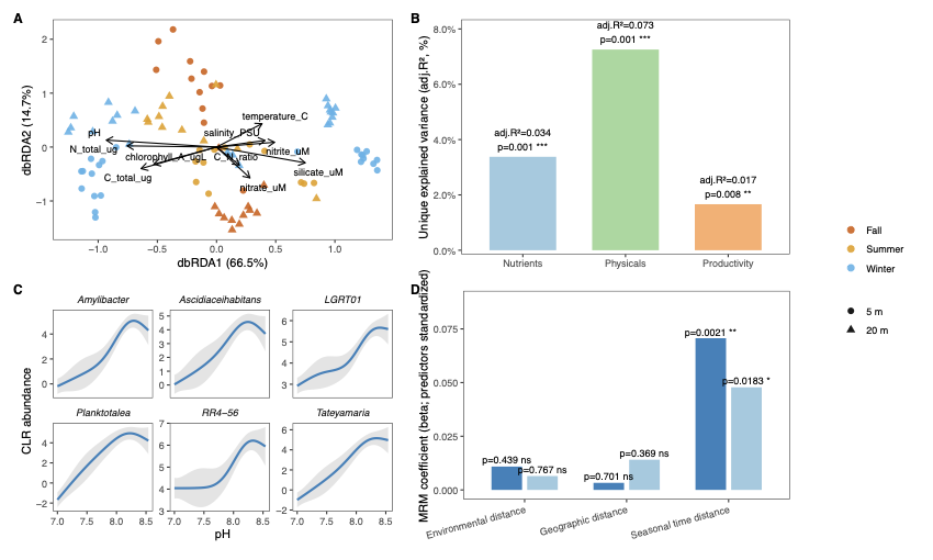
Figure 3 — What are they doing?
Script: Figure3_final.R — also writes fig3_shared_objects.RDS, which Figures 4 and 5 read.
Taxonomy tells us who is there; this figure asks what those organisms are doing by quantifying abundance-weighted functional potential from the DRAM gene annotation matrix.
MAG × gene matrix reconciliation
The hits matrix covers 677 MAGs (the full, pre-dereplication set); the phyloseq object holds 513 dereplicated MAGs. Always intersect before any analysis so you are working with the same organisms in both matrices.
source("utils.R")
library(vegan); library(ape)

ps      <- load_ps()
H_tbl   <- readr::read_csv("gene_bin_mat.collapsed.v6.csv", show_col_types=FALSE)
genes   <- H_tbl$gene
H_mat   <- as.matrix(H_tbl[, setdiff(names(H_tbl), "gene")])
rownames(H_mat) <- genes

otu       <- as(otu_table(ps), "matrix")
A_counts  <- if (taxa_are_rows(ps)) t(otu) else otu   # samples × MAGs
row_sums  <- rowSums(A_counts); row_sums[row_sums == 0] <- 1
A_rel     <- sweep(A_counts, 1, row_sums, "/")

MAG_common <- intersect(colnames(A_rel), colnames(H_mat))
A_rel_use  <- A_rel[,  MAG_common, drop=FALSE]   # samples × M
H_use      <- H_mat[,  MAG_common, drop=FALSE]   # genes   × M
# 513 MAGs in ps → intersection with 677-MAG annotation set

message(sprintf("Intersection: %d MAGs", length(MAG_common)))
Abundance-weighted functional potential
We combine the abundance matrix A (samples × MAGs) with the hit matrix H (genes × MAGs) to produce per-sample gene potentials P = A Hᵀ (samples × genes). This converts “this genome has this gene” into “this process is being performed at approximately this rate, given how abundant that genome is.”
P_raw <- A_rel_use %*% t(H_use)   # samples × genes
P_raw <- as.matrix(P_raw); colnames(P_raw) <- rownames(H_use)

# Row-normalize (compositional fingerprint per sample)
row_tot <- rowSums(P_raw); P_rel <- sweep(P_raw, 1, ifelse(row_tot==0,1,row_tot), "/")

# Hellinger transform for ordination
gene_cols <- colnames(P_rel)
P_hell    <- vegan::decostand(P_rel, method="hellinger")
Pathway dictionary and pathway totals
pathway_dict <- list(
  Respiration_ETC = c("CydA","CyoA","CoxA","CcoN","NuoF","FrdA","SdhA","AtpA","FCC"),
  Carbon_core     = c("RbcL","PEPC","AcnB","CA","CoxL","MDH"),
  B12_cobalamin   = c("BluB","BtuCDF","CobA","CobC","CobU","CbiG","IsiB"),
  DMSP_Methyl     = c("dmdA","dmdB","dmdD","dddL","DddP","mddA","dmoA","Tmm","mtoX","dorA"),
  Nitrogen_cycle  = c("AmoA","AmoB","AmoC","NxrA","NapA","NarG","NirK","NirS","NrfA","NorB","NosZ"),
  Sulfur_cycle    = c("Sqr","SoxB","DsrA"),
  Methane_redox   = c("PmoA","Mcr"),
  Phototrophy     = c("PsaA","PsbA","RHO"),
  Hydrogenases    = c("NiFe"),
  Detox_misc      = c("ArsC","RdhA","ARO","FdhA")
)
avail <- function(g) intersect(g, colnames(P_raw))

# Per-sample pathway totals from P_raw
sd        <- as.data.frame(sample_data(ps))
season_vec <- sd$season
P_raw_tbl <- tibble::as_tibble(P_raw, rownames="sample") %>%
  mutate(season = season_vec, .after="sample")

pathway_totals <- tibble(sample=P_raw_tbl$sample, season=P_raw_tbl$season)
for (nm in names(pathway_dict))
  pathway_totals[[nm]] <- rowSums(P_raw_tbl[, avail(pathway_dict[[nm]]), drop=FALSE])
Identifying sentinel genes by ω²
For each pathway, sentinel genes are those with the highest ω² effect size across seasons — the genes that carry the most seasonal signal.
compute_effect <- function(df) {
  fit <- aov(val ~ season, data=df)
  sm  <- summary(fit)[[1]]
  ss  <- sm[,"Sum Sq"]; ms <- sm[,"Mean Sq"]
  omega2 <- max((ss[1] - sm[1,"Df"]*ms[2]) / (sum(ss) + ms[2]), 0)
  tibble(F=sm[1,"F value"], p=sm[1,"Pr(>F)"], omega2=omega2)
}

gene_effects <- P_raw_tbl %>%
  pivot_longer(-c(sample,season), names_to="gene", values_to="val") %>%
  group_by(gene) %>% group_modify(~ compute_effect(.x)) %>% ungroup() %>%
  mutate(p_adj = p.adjust(p, method="BH")) %>%
  arrange(desc(omega2))

pathway_lookup <- tibble::enframe(pathway_dict, name="pathway", value="gene") %>%
  tidyr::unnest_longer(gene) %>%
  dplyr::semi_join(gene_effects, by="gene")

sentinels <- gene_effects %>%
  inner_join(pathway_lookup, by="gene") %>%
  group_by(pathway) %>%
  arrange(desc(omega2), .by_group=TRUE) %>%
  slice_head(n=3) %>% ungroup()
Key findings
| Pathway | Sentinel gene(s) | Peak season | ω² |
|---|---|---|---|
| Methane redox | mcrA | Summer | 0.41–0.42 |
| Sulfur cycling | dsrA, sqr | Fall | 0.44–0.48 |
| B₁₂/cobalamin | bluB, cobU | Fall | 0.32–0.35 |
| Photosystem II | psbA | Winter | 0.41 |
| Nitrogen cycle | — | Weak | 0.08 |
| Phototrophy (rhodopsins) | — | None | ≈ 0 |
The Winter psbA peak coincides with the Cyanobacteria bloom in Figure 1. The Fall enrichment of sulfur and B₁₂ genes likely reflects remineralisation of summer-bloom biomass, consistent with phytoplankton–bacteria coupling in Patagonian fjords Montero et al. 2011.
Panels A–D and export
main_pathways <- c("Methane_redox","Carbon_core","Sulfur_cycle","B12_cobalamin","Nitrogen_cycle")
meta_samp <- as(sample_data(ps), "data.frame") %>%
  tibble::rownames_to_column("sample") %>% dplyr::select(sample, season, depth_m)

# Panel A: pathway totals by season × depth
ptA <- pathway_totals %>%
  pivot_longer(-c(sample,season), names_to="pathway", values_to="potential") %>%
  left_join(meta_samp, by=c("sample","season")) %>%
  filter(pathway %in% main_pathways) %>%
  mutate(season=factor(season, levels=c("Summer","Fall","Winter")),
         depth_m=factor(as.character(depth_m), levels=c("5","20")))

panelA_summary <- ptA %>%
  group_by(pathway, season, depth_m) %>%
  summarise(mean=mean(potential,na.rm=TRUE), se=sd(potential,na.rm=TRUE)/sqrt(n()), .groups="drop")

# Panel C: sentinel gene z-score heatmap (see script for full sentinel_long construction)
# Panel D: PCoA on Hellinger-transformed P_rel
dist_h   <- dist(P_hell, method="euclidean")
pcoa_res <- ape::pcoa(dist_h)
scores   <- as.data.frame(pcoa_res$vectors[, 1:2])
colnames(scores)[1:2] <- c("Axis.1","Axis.2")
scores$sample <- rownames(scores)
scores <- dplyr::left_join(scores, meta_samp, by="sample")

# PERMANOVA on functional PCoA
adonis2(P_hell ~ season * depth_m, data=meta_samp, permutations=999, method="euclidean", by="margin")
# season R² ≈ 0.18, depth R² ≈ 0.10

# Save shared objects for Figures 4 and 5
saveRDS(list(A_rel_use=A_rel_use, H_use=H_use,
             pathway_dict=pathway_dict, main_pathways=main_pathways),
        "fig3_shared_objects.RDS")

ggsave("Figure3.pdf", final_fig3, width=12, height=10, units="in", device=cairo_pdf)
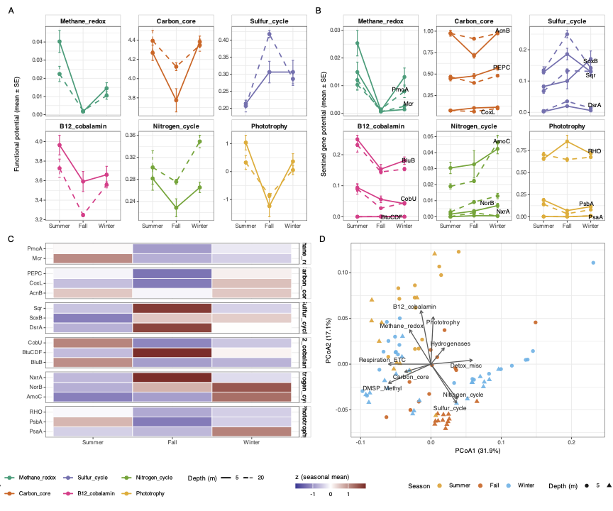
Figure 4 — Which lineages carry which functions?
Script: Figure4_final.R
We know what functions are enriched in each season (Figure 3); now we ask which families are responsible by laying functional potential onto the phylogeny. This requires collapsing the MAG phylogeny to family level and computing per-family pathway z-scores.
Load shared objects and build per-MAG pathway potentials
source("utils.R")
library(ggtree); library(ggtreeExtra); library(ggnewscale)

ps <- load_ps()
if (!exists("A_rel_use")) {
  fig3 <- readRDS("fig3_shared_objects.RDS")
  list2env(fig3, envir=.GlobalEnv)
}

fig3_paths  <- unique(c(main_pathways, "Phototrophy"))
gene_cols_H <- rownames(H_use)
avail       <- function(g) intersect(g, gene_cols_H)
mag_ids     <- colnames(H_use)

# Per-MAG pathway hit counts
mag_path_hits <- do.call(cbind, lapply(fig3_paths, function(pw) {
  gg <- avail(pathway_dict[[pw]])
  if (length(gg)==0) return(rep(0, length(mag_ids)))
  colSums(H_use[gg, , drop=FALSE], na.rm=TRUE)
}))
colnames(mag_path_hits) <- fig3_paths; rownames(mag_path_hits) <- mag_ids

# Weight by mean MAG relative abundance across all samples
mag_mean_abund     <- colMeans(A_rel_use, na.rm=TRUE)
mag_path_potential <- sweep(mag_path_hits, 1, mag_mean_abund[rownames(mag_path_hits)], `*`)
Collapse to family level, compute z-scores
tx      <- as.data.frame(tax_table(ps))
mag_tax <- tx %>% tibble::rownames_to_column("MAG_id") %>%
  dplyr::select(MAG_id, Family, Phylum) %>%
  dplyr::filter(MAG_id %in% rownames(mag_path_potential))

fam_path_potential <- mag_tax %>%
  dplyr::select(MAG_id, Family) %>%
  left_join(as.data.frame(mag_path_potential) %>% tibble::rownames_to_column("MAG_id"),
            by="MAG_id") %>%
  group_by(Family) %>%
  summarise(across(all_of(fig3_paths), ~sum(.x, na.rm=TRUE)), .groups="drop")

# Collapse phylogeny to Family
ps_fam  <- tax_glom(ps, taxrank="Family", NArm=TRUE)
fam_vec <- as.character(tax_table(ps_fam)[, "Family"])
fam_vec[is.na(fam_vec) | fam_vec==""] <- "Unassigned_Family"
taxa_names(ps_fam) <- make.unique(fam_vec, sep="__")

td      <- as.treedata(phy_tree(ps_fam))
tip_map <- tibble(
  Tip    = taxa_names(ps_fam),
  Family = as.character(tax_table(ps_fam)[,"Family"]),
  Phylum = as.character(tax_table(ps_fam)[,"Phylum"])
) %>%
  mutate(Family = if_else(is.na(Family)|Family=="","Unassigned_Family",Family),
         Phylum = if_else(is.na(Phylum)|Phylum=="","Other",Phylum))

# Build tip × pathway matrix and z-score column-wise
heat_mat <- tip_map %>%
  left_join(fam_path_potential, by="Family") %>%
  arrange(match(Tip, td@phylo$tip.label)) %>%
  dplyr::select(all_of(c("Tip", fig3_paths))) %>%
  tibble::column_to_rownames("Tip")

safe_z <- function(x) {
  x[is.na(x)] <- 0; s <- sd(x, na.rm=TRUE)
  if (!is.finite(s) || s==0) return(rep(0, length(x)))
  (x - mean(x, na.rm=TRUE)) / s
}
heat_scaled <- as.data.frame(apply(heat_mat, 2, safe_z))
colnames(heat_scaled) <- gsub("_"," ", colnames(heat_scaled))
z_lim <- max(1.5, as.numeric(quantile(abs(unlist(heat_scaled)), 0.98, na.rm=TRUE)))
Plot: circular tree + geom_fruit heatmap ring
geom_fruit from ggtreeExtra is used instead of gheatmap because it handles circular layouts correctly without conflicting with ggplot2’s coordinate system. new_scale_fill() from ggnewscale separates the Phylum colour scale from the heatmap fill scale.
heat_long <- heat_scaled %>%
  tibble::rownames_to_column("Tip") %>%
  pivot_longer(-Tip, names_to="Pathway", values_to="z_score") %>%
  mutate(Pathway = factor(Pathway, levels=colnames(heat_scaled)))

p_out <- ggtree(td, layout="circular", linewidth=0.3) %<+% tip_map +
  geom_tippoint(aes(color=Phylum), size=2.5, alpha=0.95) +
  scale_color_manual(values=pal_phylum, na.value="#BFBFBF", name="Phylum") +
  geom_tiplab2(aes(label=Family), size=2.7, offset=0.07) +
  new_scale_fill() +                         # reset fill scale for heatmap
  geom_fruit(
    data    = heat_long,
    geom    = geom_tile,
    mapping = aes(y=Tip, x=Pathway, fill=z_score),
    offset  = 0.15,   # gap between tip labels and heatmap ring
    pwidth  = 0.58,   # heatmap ring width relative to tree radius
    axis.params = list(axis="x", text.angle=45, text.size=3, hjust=0),
    grid.params = list(linetype="blank")
  ) +
  scale_fill_gradient2(low="#313695", mid="white", high="#A50026",
                       midpoint=0, limits=c(-z_lim, z_lim), oob=scales::squish,
                       name="Pathway enrichment
(family z-score)") +
  theme(legend.position="right")

ggsave("Figure4.pdf", p_out, width=450, height=400, units="mm")
Key findings
- Rhodobacteraceae: carbon core z = 7.53, sulfur z = 2.12 — broad multifunctionality; known to dominate responses to phytoplankton exudates in Patagonian fjords Valdés-Castro et al. 2022
- Flavobacteriaceae: B₁₂ z = 7.94, carbon z = 6.64 — organic matter processing specialists; keystone taxa in benthic networks under aquaculture pressure Zárate et al. 2025
- Thioglobaceae: sulfur z = 0.92 — sulfur oxidisers first identified in Comau’s chemosynthetic mats Ugalde et al. 2013
- Planctomycetaceae / Pirellulaceae: consistently below average across all pathways
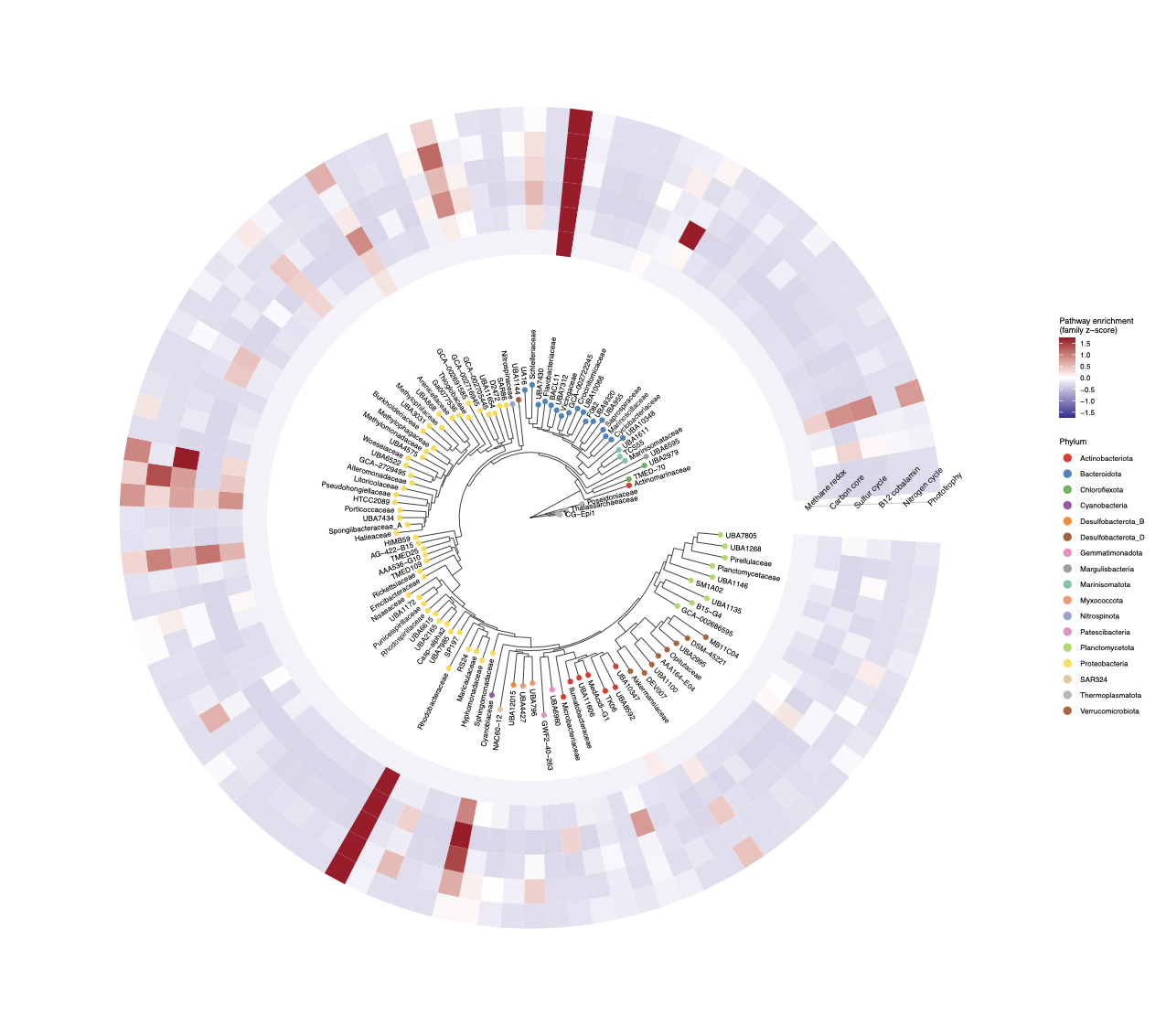
Figure 5 — How are communities assembled?
Script: Figure5_final.R
Figures 1–4 describe what communities look like and why they vary. Figure 5 addresses the mechanistic question: do communities form by chance, or is there a directional force (competition or filtering) at work? The answer differs strikingly between depths.
Standardised effect sizes (SES) — the logic
Raw diversity metrics conflate signal with richness. SES removes this dependence by comparing observed values to a null distribution from permuted communities:
SES = (observed − mean(null)) / sd(null)
| SES | Ecological interpretation |
|---|---|
| > 0 | Community is more diverse than random → limiting similarity / niche partitioning |
| ≈ 0 | No departure from random assembly |
| < 0 | Community is less diverse than random → habitat filtering |
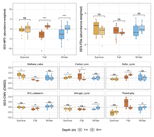
Panel A — SES-MPD (phylogenetic assembly)
Two null models are used to bracket the result. The richness null preserves per-sample species richness; the frequency null additionally preserves species-level occurrence frequencies across samples. Agreement between both nulls strengthens inference.
source("utils.R"); library(picante); library(parallel)
ps <- load_ps()
if (!exists("A_rel_use")) { fig3 <- readRDS("fig3_shared_objects.RDS"); list2env(fig3, envir=.GlobalEnv) }

set.seed(123); runs <- 999

# Community matrix (samples × taxa), relative abundances
otu       <- as(otu_table(ps), "matrix")
comm_counts <- if (taxa_are_rows(ps)) t(otu) else otu
comm_rel  <- sweep(comm_counts, 1, rowSums(comm_counts), "/"); comm_rel[is.na(comm_rel)] <- 0

# Rarity filter: drop taxa with prevalence < 2 AND max RA < 1e-4
keep_taxa <- colSums(comm_rel > 0) >= 2 | apply(comm_rel, 2, max) >= 1e-4
comm_rel  <- comm_rel[, keep_taxa, drop=TRUE]

# Align tree and community
phy  <- phy_tree(ps)
mp   <- picante::match.phylo.comm(phy, comm_rel)
Dphy <- ape::cophenetic.phylo(mp$phy)

# Parallel SES-MPD runner (uses mclapply on Unix; parLapply on Windows)
run_ses_parallel <- function(comm, D, null_model, runs, ncores=NA_integer_) {
  n      <- nrow(comm)
  cores  <- if (is.na(ncores)) max(1L, min(parallel::detectCores(TRUE)-1L, 8L)) else as.integer(ncores)
  blocks <- split(seq_len(n), ceiling(seq_along(seq_len(n)) / ceiling(n/cores)))
  run_block <- function(idx)
    picante::ses.mpd(mp$comm[idx,,drop=FALSE], D, null.model=null_model,
                     runs=runs, abundance.weighted=TRUE)
  if (.Platform$OS.type == "windows") {
    cl <- parallel::makeCluster(cores)
    on.exit(parallel::stopCluster(cl), add=TRUE)
    parallel::clusterEvalQ(cl, library(picante))
    res <- parallel::parLapply(cl, blocks, run_block)
  } else {
    res <- parallel::mclapply(blocks, run_block, mc.cores=cores)
  }
  dplyr::bind_rows(lapply(res, function(r) { r$sample <- rownames(r); tibble::as_tibble(r) }))
}

meta_aln <- as(sample_data(ps), "data.frame") %>%
  tibble::rownames_to_column("sample") %>%
  dplyr::filter(sample %in% rownames(mp$comm)) %>%
  mutate(season  = factor(season,  levels=c("Summer","Fall","Winter")),
         depth_m = factor(as.character(depth_m), levels=c("5","20")))

ses_rich <- run_ses_parallel(mp$comm, Dphy, "richness",  runs) %>% left_join(meta_aln, by="sample")
ses_freq <- run_ses_parallel(mp$comm, Dphy, "frequency", runs) %>% left_join(meta_aln, by="sample")
Panel B — SES-FDis (functional dispersion)
FDis is the abundance-weighted mean distance of each organism to the community-weighted centroid in trait space. The trait space is defined by log1p-standardised pathway hit counts across the six Figure 3 pathways. Because there is no standard null for FDis, we implement permutation-based SES directly.
# Trait matrix: log1p + column-standardise pathway hits
fig3_paths <- unique(c(main_pathways, "Phototrophy"))
mag_ids    <- colnames(H_use)
avail      <- function(g) intersect(g, rownames(H_use))

mag_path_hits <- do.call(cbind, lapply(fig3_paths, function(pw) {
  gg <- avail(pathway_dict[[pw]])
  if (length(gg)==0) return(rep(0, length(mag_ids)))
  colSums(H_use[gg,,drop=FALSE], na.rm=TRUE)
}))
colnames(mag_path_hits) <- fig3_paths; rownames(mag_path_hits) <- mag_ids

comm   <- A_rel_use[meta_aln$sample,, drop=FALSE]
traits_raw <- mag_path_hits[intersect(colnames(comm), rownames(mag_path_hits)),,drop=FALSE]
comm       <- comm[, rownames(traits_raw), drop=FALSE]
traits_use <- scale(log1p(traits_raw)); traits_use[is.na(traits_use)] <- 0
traits_use <- traits_use[, apply(traits_use,2,sd)>0, drop=FALSE]

# Fast abundance-weighted FDis
fast_fdis <- function(comm, traits) {
  W <- comm / rowSums(comm); T <- as.matrix(traits); C <- W %*% T
  vapply(seq_len(nrow(W)), function(s) {
    cs <- as.numeric(C[s,]); dev <- sweep(T,2,cs,"-")
    sum(W[s,] * sqrt(rowSums(dev^2)))
  }, numeric(1))
}

Fobs   <- fast_fdis(comm, traits_use)
Fnull  <- replicate(999, fast_fdis(comm, traits_use[sample(nrow(traits_use)),,drop=FALSE]))
SES_FDis <- (Fobs - rowMeans(Fnull)) / apply(Fnull,1,sd)

dfC <- tibble(sample=rownames(comm), SES_FDis=as.numeric(SES_FDis)) %>%
  left_join(meta_aln, by="sample") %>%
  filter(!is.na(season), !is.na(depth_m), is.finite(SES_FDis))
Panel C — SES-CWSD (per-pathway functional dispersion)
SES-CWSD extends FDis to each trait axis individually, showing which specific pathways are over- or under-dispersed within communities.
# CWSD: per-trait standard deviation weighted by abundance
C_obs  <- (comm / rowSums(comm)) %*% as.matrix(traits_use)
CWSD_obs <- t(vapply(seq_len(nrow(comm)), function(s) {
  cs  <- as.numeric(C_obs[s,]); W <- comm[s,] / sum(comm[s,])
  dev <- sweep(as.matrix(traits_use), 2, cs, "-")
  sqrt(colSums(W * (dev^2)))
}, numeric(ncol(traits_use))))
rownames(CWSD_obs) <- rownames(comm)

# Null: permute MAG trait labels 999 times (frequency null)
set.seed(123)
null_cwsd <- replicate(999, {
  T_perm <- as.matrix(traits_use)[sample(nrow(traits_use)),,drop=FALSE]
  C_p <- (comm / rowSums(comm)) %*% T_perm
  t(vapply(seq_len(nrow(comm)), function(s) {
    cs <- as.numeric(C_p[s,]); W <- comm[s,] / sum(comm[s,])
    dev <- sweep(T_perm, 2, cs, "-")
    sqrt(colSums(W * (dev^2)))
  }, numeric(ncol(traits_use))))
}, simplify="array")   # samples × traits × 999

mu_null <- apply(null_cwsd, c(1,2), mean)
sd_null <- apply(null_cwsd, c(1,2), sd); sd_null[sd_null==0] <- 1
SES_CWSD <- (CWSD_obs - mu_null) / sd_null

dfD <- as.data.frame(SES_CWSD) %>%
  tibble::rownames_to_column("sample") %>%
  pivot_longer(-sample, names_to="trait", values_to="SES_CWSD") %>%
  left_join(meta_aln, by="sample") %>%
  filter(!is.na(season), !is.na(depth_m), is.finite(SES_CWSD))
Assembly and export
library(patchwork)
fig5 <- (p_freq + labs(title=NULL)) +          # Panel A: SES-MPD (frequency null)
        (p_4C   + labs(title=NULL)) +           # Panel B: SES-FDis
        (p_4D   + labs(title=NULL)) +           # Panel C: SES-CWSD per pathway
  plot_layout(design="AB
CC", guides="collect") &
  theme(legend.position="bottom")

ggsave("Figure5.pdf", fig5, width=180, height=160, units="mm", device=cairo_pdf)
Key findings
- 5 m, Summer and Winter: SES-MPD ≈ +4 to +6, SES-FDis > +1.5 → limiting similarity dominates at the surface
- 20 m, Winter: SES-MPD < −5 → strong habitat filtering at depth
- Phototrophy at 5 m (Summer/Fall): SES-CWSD > +2 → many phylogenetically distant lineages share phototrophic potential, consistent with competition for light
This depth-dependent contrast in assembly mechanisms is consistent with long-term time-series evidence that surface and near-seafloor communities show the strongest seasonal signals while intermediate depths are more temporally stable Cram et al. 2014.
Anthropogenic context and conservation relevance
The microbial dynamics documented here are embedded in a system under three overlapping pressures:
1. Salmon aquaculture — nutrient loading, salmon feed DOM, and antibiotic use alter bacterioplankton composition and function Olsen et al. 2017; Montero et al. 2022. Communities already carry elevated ARGs Guajardo-Leiva et al. 2023.
2. Harmful algal blooms — the same seasonal forcing driving natural community dynamics can trigger catastrophic events under anomalous atmospheric conditions, as documented by the 2021 Heterosigma akashiwo bloom that killed ~6,000 tonnes of farmed salmon Díaz et al. 2022.
3. Climate change — rising surface temperatures threaten to reduce microbial diversity by eliminating key taxa (Flavobacteriaceae, Rhodobacteraceae, Cenarchaeaceae) central to organic matter cycling Gutiérrez et al. 2018. Reduced glacier melt would lower silicon supply, potentially shifting phytoplankton communities from diatoms toward non-silicified taxa with downstream bacterioplankton effects Olsen et al. 2014.
The baseline community dynamics described here provide the reference state against which all of these perturbations can be evaluated.
Adapting this workflow to your own data
The core pipeline is general to any MAG or OTU-based metagenomics study:
| What to change | Where |
|---|---|
Point load_ps() to your phyloseq object | utils.R |
Update pal_phylum with your phyla | utils.R |
| Replace the gene hit matrix | gene_bin_mat.collapsed.v6.csv — column names must match MAG IDs in the phyloseq object |
| Update sentinel gene lists | pathway_dict in Figure3_final.R |
| Change season boundaries (Northern Hemisphere) | get_season_sh in utils.R |
| Use a different gradient axis instead of depth | Replace depth_m throughout — any two-level environmental factor works |
References
A First Insight into the Microbial and Viral Communities of Comau Fjord — Guajardo-Leiva et al., 2023, Microorganisms
Spatially and Temporally Explicit Metagenomes and MAGs from the Comau Fjord — Castro-Nallar et al., 2023, Microbiology Resource Announcements
Microbial Life in a Fjord: Metagenomic Analysis of a Microbial Mat — Ugalde et al., 2013, PLoS ONE
Responses in bacterial community structure to waste nutrients from aquaculture — Olsen et al., 2017, Aquaculture Environment Interactions
Responses in the microbial food web to increased rates of nutrient supply — Olsen et al., 2014, Aquaculture Environment Interactions
The Effect of Salmon Food-Derived DOM and Glacial Melting on Bacterioplankton — Montero et al., 2022, Frontiers in Microbiology
Capturing the spatial structure of the benthic microbiome under aquaculture — Zárate et al., 2025, BMC Microbiology
The impact of local and climate change drivers on HAB formation in a Patagonian fjord — Díaz et al., 2022, Science of the Total Environment
Linking Seasonal Reduction of Microbial Diversity to Winter Temperature — Gutiérrez et al., 2018, Frontiers in Marine Science
Influence of Estuarine Water on the Microbial Community Structure of Patagonian Fjords — Tamayo-Leiva et al., 2021
Seasonal variability of primary production in a Patagonian fjord — Montero et al., 2011, Continental Shelf Research
Assessment of Microbial Community Composition Changes with Phytoplankton-Derived Exudates — Valdés-Castro et al., 2022, Diversity
Seasonal and diel variations in zooplankton in Comau Fjord — Garcia-Herrera et al., 2022, PeerJ
Depth-Dependent Diversity Patterns in Comau Fjord — Villalobos et al., 2021
Exploring the Diversity and Antimicrobial Potential of Marine Actinobacteria from Comau Fjord — Undabarrena et al., 2016, Frontiers in Microbiology
Seasonal and interannual variability of marine bacterioplankton throughout the water column — Cram et al., 2014, The ISME Journal
Session info
sessioninfo::session_info()
Save this output alongside your figures. Bioconductor packages (phyloseq, ggtree, ggtreeExtra) evolve rapidly and version mismatches are the most common source of non-reproducibility.